Usage
Load Data in QGIS
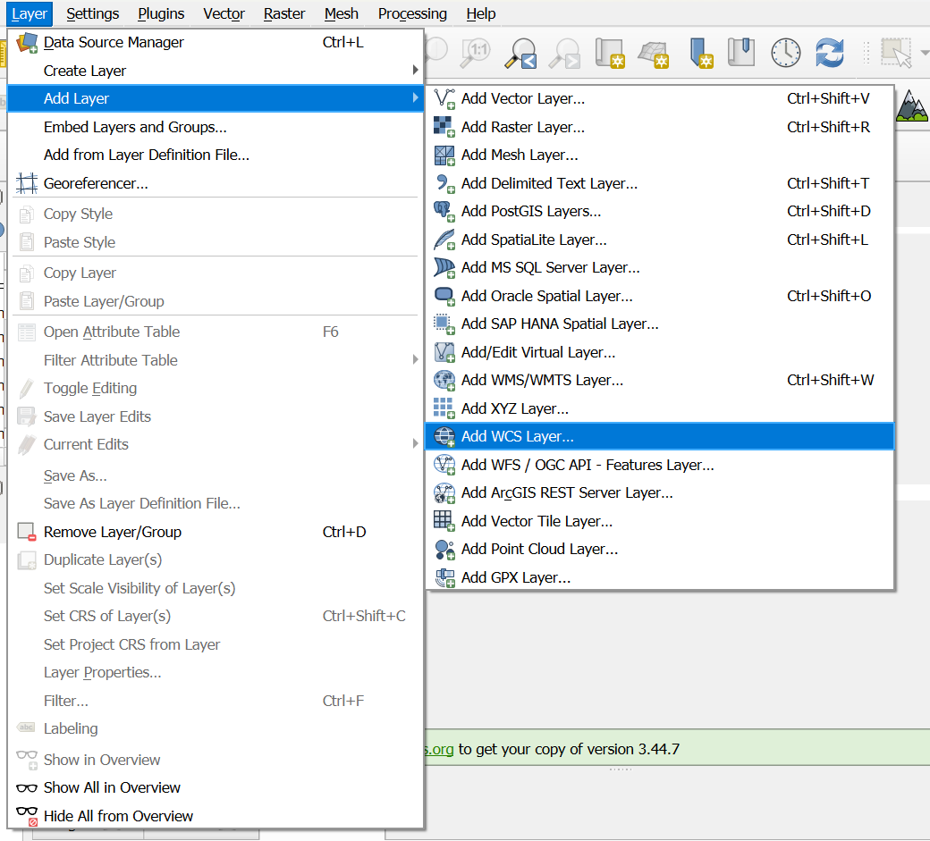
The PDC layers are accessible in QGIS via the top menu. Click on “Layer/Add Layer/Add WCS Layer”:
A new window should open. In the “Layers” tab, click on “New”. This should open another window to create the new WCS connection.
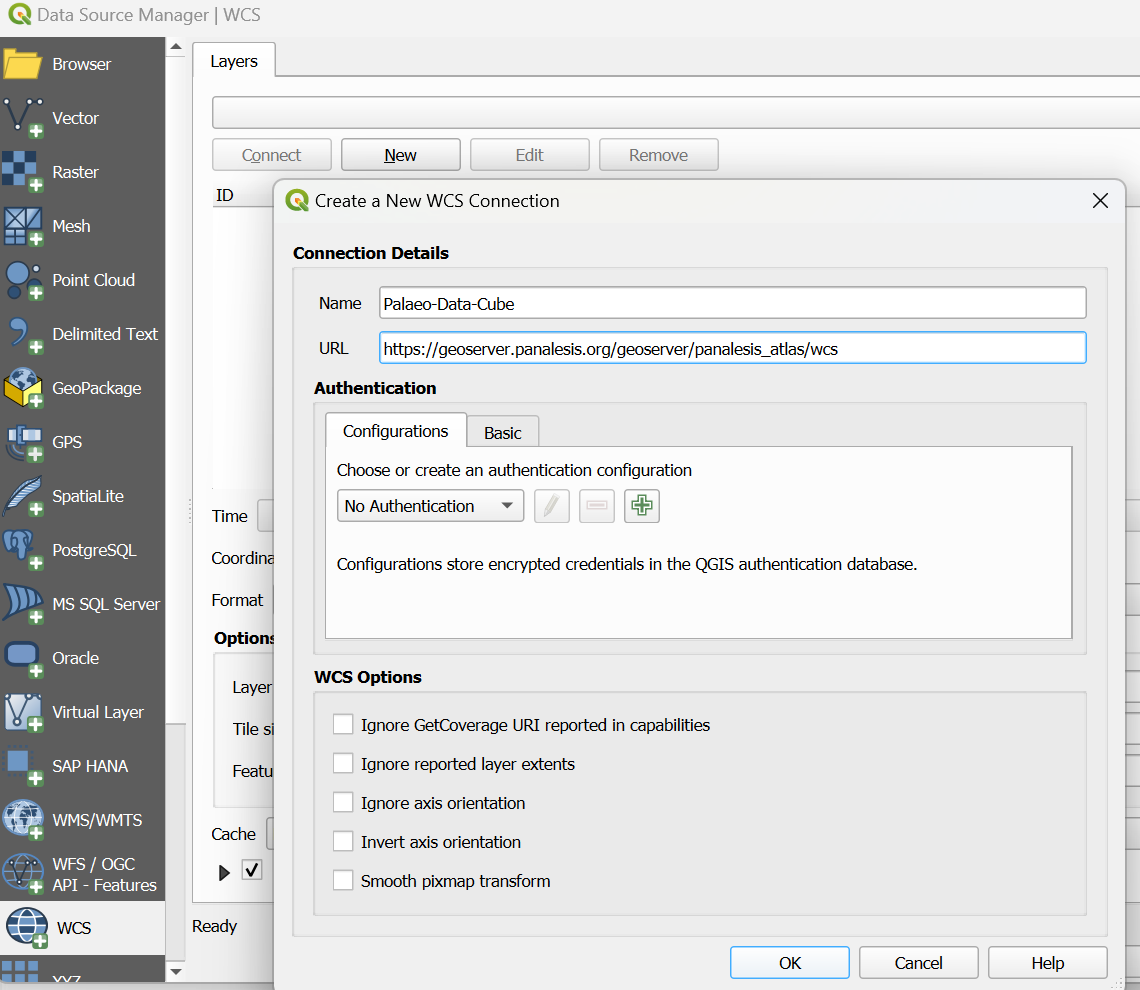
Fill in the information: for the name, anything like “Palaeo Data Cube” is fine. Depending on the layers you want, the URL should be :
For equal area: https://geoserver.panalesis.org/geoserver/panalesis_atlas/wcs
For lat/lon: https://geoserver.panalesis.org/geoserver/panalesis_atlas_epsg_4326/wcs
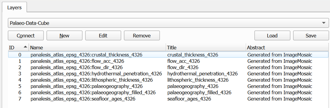
Click on “OK”, and then on “Connect”. All layers should be listed:
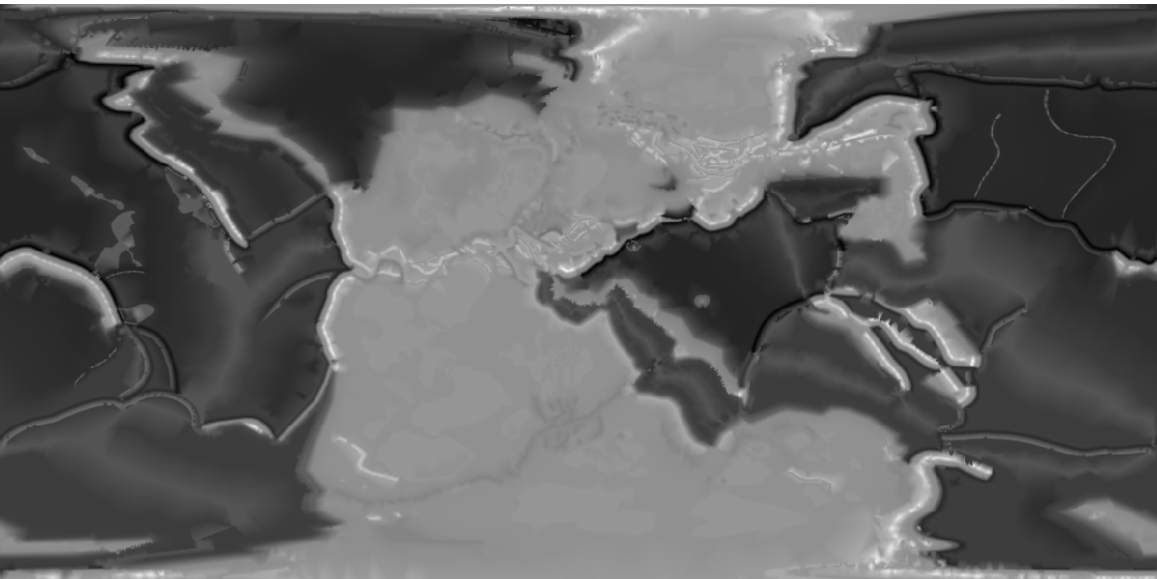
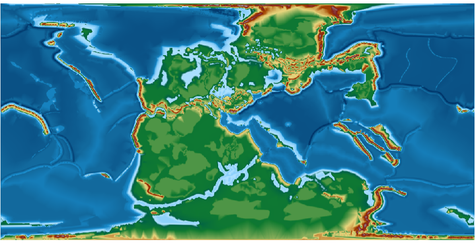
Clicking on one of the layers will allow you to select a time-step. The format follows the ISO 8601 format explained before, with the geological age being embedded by adding 2000 to it, so 250 Ma would be ‘2250-01-01T00:00:00.000Z’. If we select this timeslice, the map should look like:
If you want to apply a pre-defined style to this layer, some .qml files are available in the files/styles folder:
https://github.com/florianfranz/palaeo-data-cube/tree/main/files/styles
Apply the palaeogeography style by downloading it from the folder, then go to QGIS, double click on the layer, go to
the symbology window and on the bottom-left, click on Styles/Load Style and browse to select the file. Load it and
click OK. The style should be applied and your map should look like this:
Load Data in Python
Discovering available time steps
Before requesting raster data via WCS, it is often useful to know which temporal
slices are available for a given layer. GeoServer exposes this information
through the WCS DescribeCoverage operation.
The following example queries the service and returns the list of available geological ages (in millions of years, Ma) for a raster layer.
import requests
from xml.etree import ElementTree as ET

def get_available_ages(
        layer_name,
        base_url="https://geoserver.panalesis.org/geoserver/",
        workspace="panalesis_atlas",
        service_type="WCS",
        service_version="1.0.0"
):
    describe_url = (
        f"{base_url}{workspace}/{service_type.lower()}"
        f"?service={service_type}&version={service_version}"
        f"&request=DescribeCoverage&coverage={workspace}:{layer_name}"
    )
    response = requests.get(describe_url)
    root = ET.fromstring(response.content)

    years = sorted(set(
        int(el.text.split("-")[0])
        for el in root.iter()
        if el.tag.endswith('timePosition') and el.text
    ))
    geological_ages = [year - 2000 for year in years]

    return years, geological_ages
The function can be called by providing a layer name:
years, geological_ages = get_available_ages("palaeogeography")
print(geological_ages)
print(f"Number of reconstructions: {len(geological_ages)}")
Example output:
[0, 6, 11, 15, 20, 33, 40, 48, 56, 68, 84, 94, 100, 113, 120, 133, 140,
 154, 165, 180, 200, 210, 220, 230, 240, 250, 270, 290, 300, 315, 331,
 350, 370, 383, 393, 408, 420, 444, 463, 475, 489, 500, 518, 535, 545]


Number of reconstructions: 45
Each value corresponds to a valid time step that can be used in subsequent WCS
GetCoverage requests.
Loading raster data via WCS
This example shows how to retrieve raster data from a Web Coverage Service (WCS) and display it using Python. Users only need to specify the layer name and the geological age.
The WCS request returns a GeoTIFF, which is read and visualized using
rasterio and matplotlib.
Example
def construct_wcs_url(layer_name,
                   geological_age,
                   base_url="https://geoserver.panalesis.org/geoserver/",
                   workspace="panalesis_atlas",
                   service_type="WCS",
                   service_version="1.0.0",
                   request_type="GetCoverage",
                   crs="EPSG:54034",
                   bbox="-20037508.34,-6363885.33,20037508.34,6363885.33",
                   resx="10000",
                   resy="10000",
                   format="GEOTIFF"):

    time = f"{geological_age + 2000:04d}-01-01T00:00:00.000Z"

    url = (
        rf"{base_url}{workspace}/{service_type.lower()}?"
        rf"service={service_type}&"
        rf"version={service_version}&"
        rf"request={request_type}&"
        rf"coverage={workspace}:{layer_name}&"
        rf"crs={crs}&"
        rf"bbox={bbox}&"
        rf"resx={resx}&"
        rf"resy={resy}&"
        rf"time={time}&"
        rf"format={format}"
    )
    return url
This function can be called simply:
geological_age = 250
layer_name = "palaeogeography"
wcs_url = construct_wcs_url(layer_name, geological_age)
print(wcs_url)
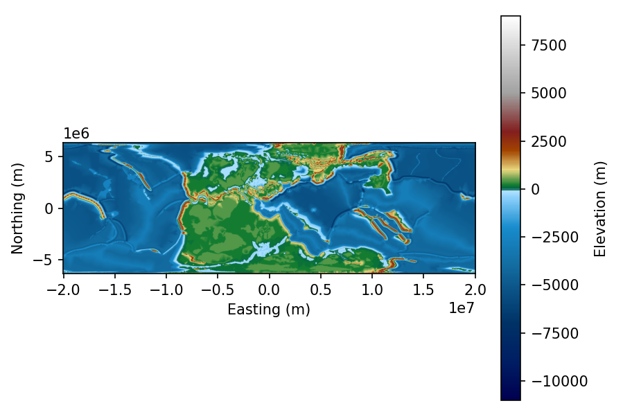
This should return a correct WCS URL like:
https://geoserver.panalesis.org/geoserver/panalesis_atlas/wcs?service=WCS&version=1.0.0&request=GetCoverage&coverage=panalesis_atlas:palaeogeography&crs=EPSG:54034&bbox=-20037508.34,-6363885.33,20037508.34,6363885.33&resx=10000&resy=10000&time=2250-01-01T00:00:00.000Z&format=GEOTIFF
You can now use this URL to load the data using requests and rasterio, then plot it with matplotlib
from rasterio.io import MemoryFile
import matplotlib.pyplot as plt
import matplotlib.colors as mcolors
import numpy as np

colormap_entries = [
    (9000, "#ffffff", "9000"),
    (7000, "#cecece", "7000"),
    (5000, "#a1a1a1", "5000"),
    (3000, "#821e1e", "3000"),
    (2000, "#a34400", "2000"),
    (1000, "#e8d67d", "1000"),
    (200, "#107b30", "200"),
    (0, "#006147", "0"),
    (-100, "#b0e2ff", "-100"),
    (-500, "#87cefa", "-500"),
    (-2000, "#188ccd", "-2000"),
    (-4000, "#136ca0", "-4000"),
    (-7000, "#003266", "-7000"),
    (-9000, "#001e64", "-9000"),
    (-11000, "#000050", "-11000"),
]

colormap_entries_sorted = sorted(
    colormap_entries,
    key=lambda x: x[0]
)
elevations = [e[0] for e in colormap_entries_sorted]
colors = [e[1] for e in colormap_entries_sorted]

vmin, vmax = elevations[0], elevations[-1]
norm_values = [(e - vmin) / (vmax - vmin) for e in elevations]
cmap = mcolors.LinearSegmentedColormap.from_list(
    "palaeogeography",
    list(zip(norm_values, colors))
)
norm = mcolors.Normalize(vmin=vmin, vmax=vmax)

data = requests.get(wcs_url).content
with MemoryFile(data) as memfile:
    with memfile.open() as dataset:
        raster = dataset.read(1).astype(float)

        nodata = dataset.nodata
        if nodata is not None:
            raster[raster == nodata] = np.nan

        bounds = dataset.bounds
        extent = [bounds.left, bounds.right, bounds.bottom, bounds.top]

        fig, ax = plt.subplots()
        img = ax.imshow(
            raster,
            cmap=cmap,
            norm=norm,
            extent=extent,
            origin="upper"
        )
        cbar = plt.colorbar(img, ax=ax)
        cbar.set_label("Elevation (m)")
        ax.set_xlabel("Easting (m)")
        ax.set_ylabel("Northing (m)")
        plt.show()
Notes
workspacecorresponds to the GeoServer workspace or data storelayer_nameis the published raster layerage_macontrols the temporal slice via the WCStimeparameterThe spatial extent and output resolution are fixed for simplicity
Filter by dimensions
It is possible to access every product, every age and, if necessary, only a subset of the spatial extent by changing the parameters in the WCS request function.
Subsetting by product
For instance, for seafloor ages, it is possible to check the available maps by calling the get_available_ages function:
years, geological_ages = get_available_ages("seafloor_ages")
print(geological_ages)
print(f"Number of reconstructions: {len(geological_ages)}")
that will return, as it did for the palaeogeography, the list of available time steps for this product:
[0, 6, 11, 15, 20, 33, 40, 48, 56, 68, 84, 94, 100, 113, 120, 133, 140,
 154, 165, 180, 200, 210, 220, 230, 240, 250, 270, 290, 300, 315, 331,
 350, 370, 383, 393, 408, 420, 444, 463, 475, 489, 500, 518, 535, 545]


Number of reconstructions: 45
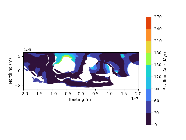
Now, plotting a map of seafloor ages for the Ordovician at 444 Ma:
geological_age = 444
layer_name = "seafloor_ages"
wcs_url = construct_wcs_url(layer_name, geological_age)
print(wcs_url)
In order to simplify the plotting process, we can define a function to plot maps that requires the WCS URL, the colormap and a title:
import requests
import numpy as np
import matplotlib.pyplot as plt
from matplotlib.colors import ListedColormap, BoundaryNorm
from rasterio.io import MemoryFile

def plot_map(wcs_url, colormap, title):
    data = requests.get(wcs_url).content
    with MemoryFile(data) as memfile:
        with memfile.open() as dataset:
            raster = dataset.read(1).astype(float)
            nodata = dataset.nodata
            if nodata is not None:
                raster = np.ma.masked_equal(raster, nodata)
            else:
                raster = np.ma.masked_invalid(raster)
            bounds = [entry[0] for entry in colormap]
            colors = [entry[1] for entry in colormap[:-1]]
            cmap = ListedColormap(colors)
            norm = BoundaryNorm(
                bounds,
                ncolors=len(colors)
            )
            cmap.set_bad(color='white')
            bounds = dataset.bounds
            extent = [
                bounds.left,
                bounds.right,
                bounds.bottom,
                bounds.top
            ]

            fig, ax = plt.subplots()
            img = ax.imshow(
                raster,
                cmap=cmap,
                norm=norm,
                extent=extent,
                origin="upper")
            cbar = plt.colorbar(img, ax=ax)
            cbar.set_label(title)
            ax.set_xlabel("Easting (m)")
            ax.set_ylabel("Northing (m)")
            plt.show()
            return raster
In our case, this can be done for the seafloor ages we defined above. We just need to add a colormap:
sf_colormap_entries = [
    (0, "#30123b", "0"),
    (30, "#4040a2", "30"),
    (60, "#4680f6", "60"),
    (90, "#25c0e7", "90"),
    (120, "#1ad2d2", "120"),
    (150, "#96fe44", "150"),
    (180, "#e9d539", "180"),
    (210, "#fe9029", "210"),
    (240, "#e2430a", "240"),
    (270, "#c52603", "270")
]
NB: Colormaps are available (.qml files for QGIS, and as lists for Python) here: https://github.com/florianfranz/palaeo-data-cube/tree/main/files/styles
seafloor_ages_url = construct_wcs_url("seafloor_ages", 444)
raster = plot_map(
    seafloor_ages_url,
    sf_colormap_entries,
    "Seafloor Age (Myr)"
)
Which should return the following map:
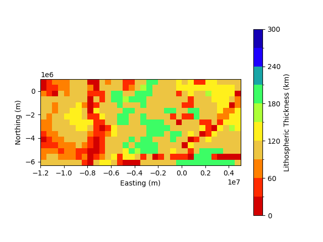
Subset by extent
Subsetting by extent can also be done by changing the bbox parameter in the function:
litho_subset = construct_wcs_url("lithospheric_thickness",
                                 140,
                                 bbox="-12000000,-6300000,5000000,1000000"
                                 )
NB: Units of the bbox follow the crs units, by default in meters.
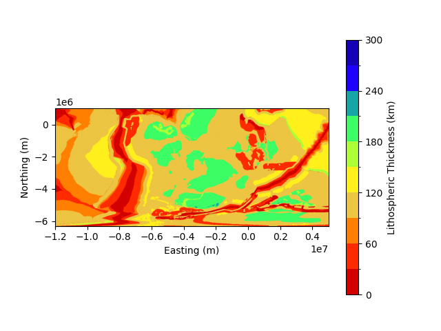
This will call the lithospheric thickness layer, for the 140 Ma reconstruction over the defined bbox.
Applying the colormap associated with lithospheric thickness and plotting:
lt_colormap_entries = [
    (0, "#d30000", "0"),
    (30, "#ff2b00", "30"),
    (60, "#ff8000", "60"),
    (90, "#edc542", "90"),
    (120, "#fff01c", "120"),
    (150, "#acff37", "150"),
    (180, "#3cfd65", "180"),
    (210, "#18a5a7", "210"),
    (240, "#1e00ff", "240"),
    (270, "#1500b6", "270"),
    (300, "#1500b6", "300"),
]

raster_litho_corner = plot_map(
    litho_subset,
    lt_colormap_entries,
    "Lithospheric Thickness (km)")
Will now render:
Change Resolution
The available layers are natively available in 10x10km resolution, and will be rendered with this resolution by default.
If you however wish to get a lower resolution, just modify the resx and resy parameters in the URL constructor:
low_res = "500000"

litho_subset_low_res = construct_wcs_url("lithospheric_thickness",
                                 140,
                                 bbox="-12000000,-6300000,5000000,1000000",
                                 resx=low_res,
                                 resy=low_res
                                 )

raster_litho_corner_low_res = plot_map(
    litho_subset_low_res,
    lt_colormap_entries,
    "Lithospheric Thickness (km)")
Will now render:
The resampling is done on the server side. By default, GeoServer will use the nearest neighbour method, taking the closest value to the new resolution pixels centroid. We therefore recommend using the native resolution.
Further Usage
We showed above the two main ways to load the data for QGIS and in Python. The purpose of this documentation is not to provide step-by-step instructions on how to use some specific layers of the Palaeo Data Cube. You may however find a full course that uses the Palaeo Data Cube at https://unige-cgeom.github.io/SPACE-GEOLOGY/. This open course provides an exercise in three parts on how to access, process, combine, visualize and export layers using Jupyter Notebooks.
The exercise is part of the SPACE-GEOLOGY (SPACE stands for Spatial Predictions and Analyses in Complex Environments) - Methods for multiscale Earth science modelling, in which we apply GIS tools to analyze the evolution of the Earth in deep-time:
Reconstructing Earth’s Past – From a Snapshot to Deep Time
How Fast Was Earth’s Engine Running?
Palaeogeography Meets Palaeoclimatology